I would like to have a conditional formatting for the last 3 columns… But once I figure how to do it in one, I’ll be able to figure out the rest I think.
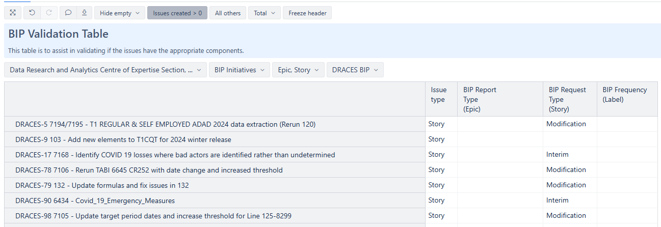
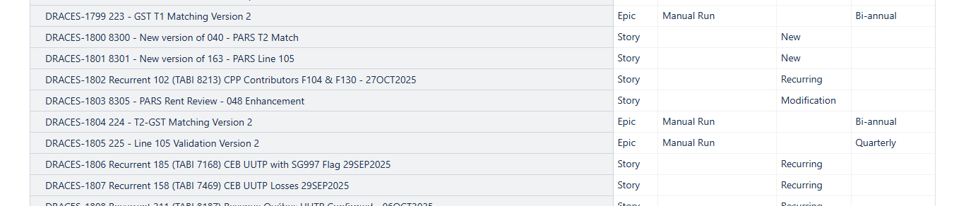
My goal is to highlight the empty cells based on the Issue type (Epic or Story) in the 1st column.
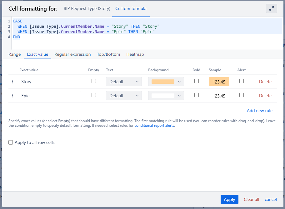
I thought that using Exact Value would work, but no colour shows:
CASE
WHEN [Issue Type].CurrentMember.Name = “Story” THEN “Story”
WHEN [Issue Type].CurrentMember.Name = “Epic” THEN “Epic”
END
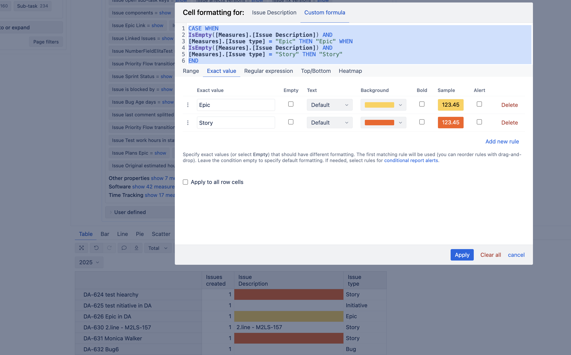
The reason your measure doesnt work is because you don’t have the Issue Type dimension in Rows, but in your custom formula, you refer to the Issue Type dimension as it would be visible in the report.
Instead, your goal is to reference the issue property “Issue Type”
Here’s an example, if you also want to highlight only those rows that are empty. As an example, I have selected the property “Issue summary”, and I only want to highlight those rows that are empty and color-code them based on the Issue type
Here’s the expression to use:
CASE
WHEN
IsEmpty([Measures].[Issue Description]) AND
[Measures].[Issue type] = "Epic"
THEN "Epic"
WHEN
IsEmpty([Measures].[Issue Description]) AND
[Measures].[Issue type] = "Story"
THEN "Story"
END