Hi,
I try to create a risk matrix in eazyBI. It should show all columns and rows at any time, no matter if there are risks in the respective cell or not.
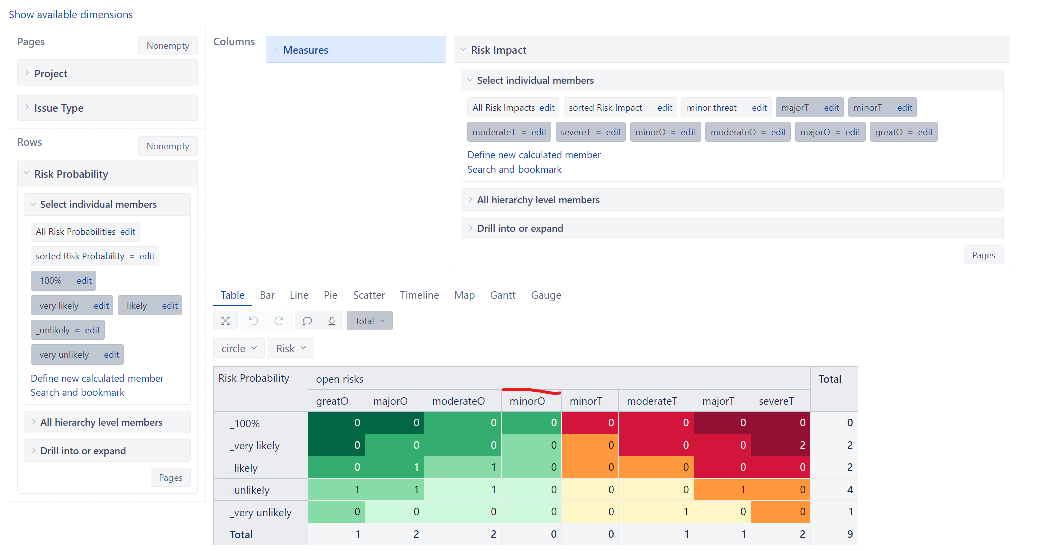
I’ve managed to get the rows and columns in the right order using calculated members:
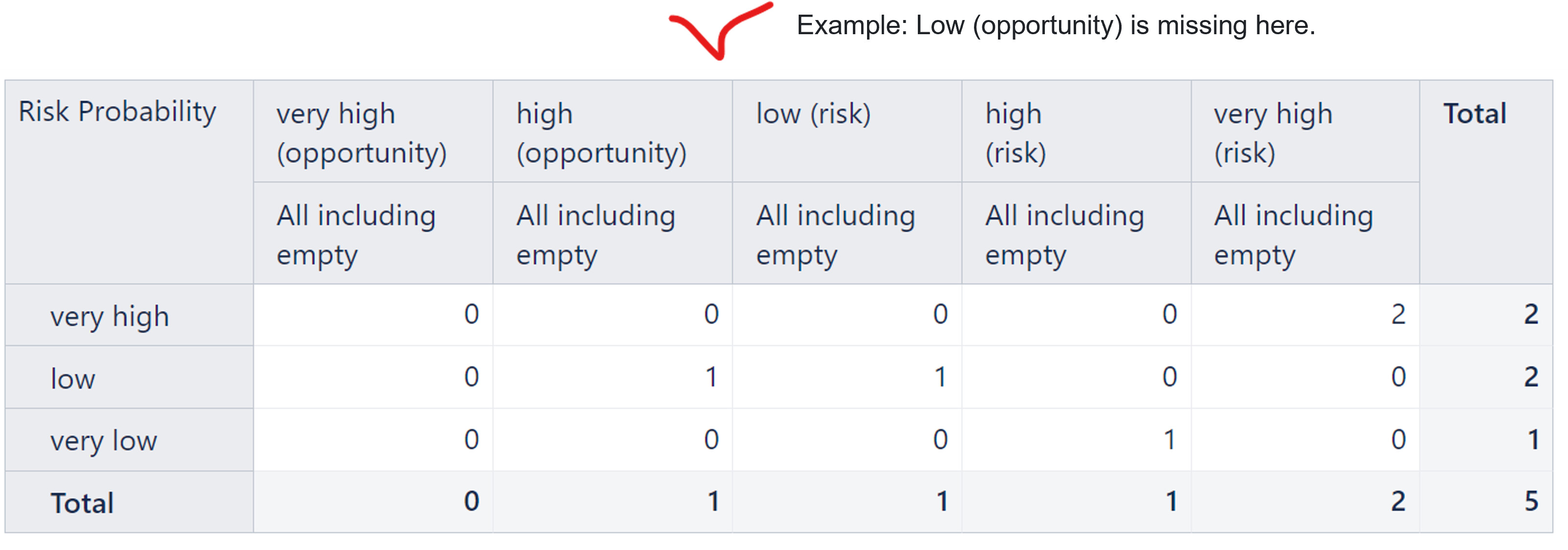
But, for example, if there is no risk with Impact “high”, the column “high (risk)” is not shown. How can i get eazyBI to show all columns and all rows at any time. If there is no issue for the cell “0” should be displayed.
I’ve tried a measure with the following code, but it just converted the empty cells to 0 for the rows and columns that were already shown.
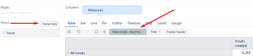
@Erik1 suggestion might indeed help (thank you, @Erik1!). If your “hide empty” option is enabled, that might be the reason you do not see any data. If this still doesn’t help, please make sure that:
You have imported all custom members into the eazyBI report
The name of all members is written correctly in your aggregate function (I suggest using autocomplete list)
Hi,
thanks for your tipps.
The settings “Nonempty” and “Hide empty columns” were already set correctly.
I think the problem is, that there is not a single issue in the data with probability=high and impact=low (opportunity).
I’ve found a workaround to define seperate calculated member for every status and add them manually to the report, but i don’t think that is the best solution.
Did you ever get a resolution for this? if you did please could you share or alternativly share the calculated measure code example for one of the individual risk levels?
Hi @Jed1003 ,
unfortunately there was no other solution.
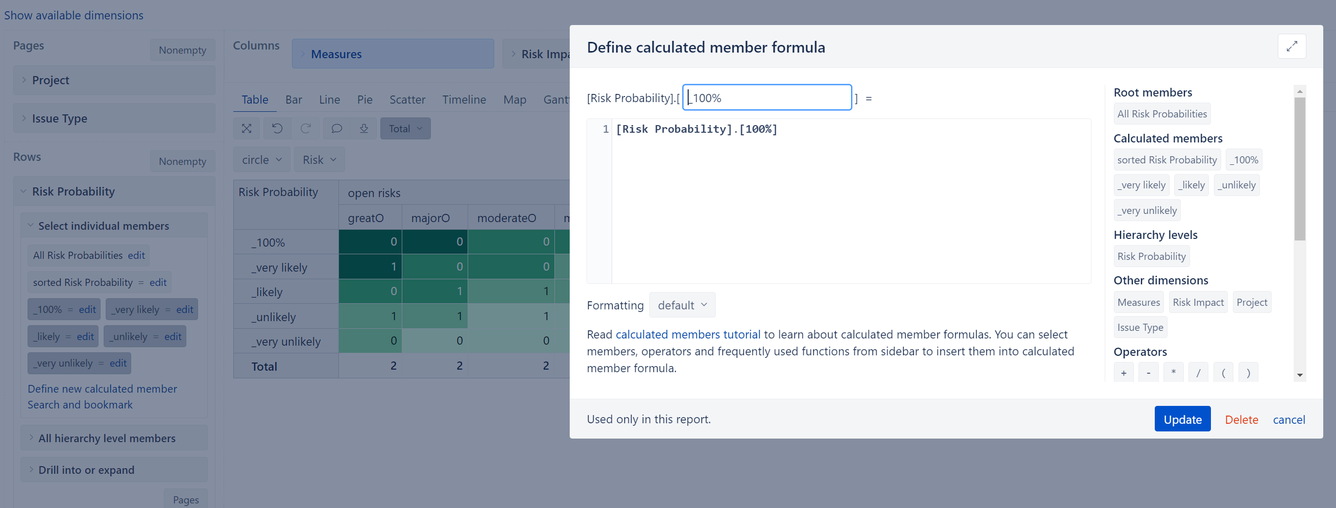
Attached you find a screenshot for one of my calculated members. Hope it helps.
Please be aware, that you cannot name the calculated member exactly like the field value. That’s why I chose to use the underscores.
Thanks @MZH . You would have thought EazyBi could do this considering Risk Matrix is a fundamental report. Many thanks for getting back to me so quickly
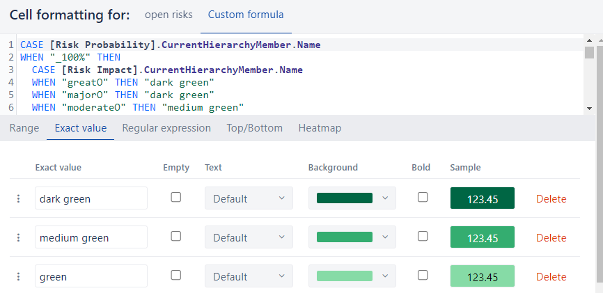
Hi @MZH - Last question i promise! How did you get the formatting? I’ve tried the conditional formatting but obvioulsy does not work with “Range” as there may be many cells in a specific row or column with the same number. Could you share how you managed this please. Thanks again!
Honestly: I don’t know if there might be a more efficient way
Best regards
Martin
CASE [Risk Probability].CurrentHierarchyMember.Name
WHEN "_100%" THEN
	CASE [Risk Impact].CurrentHierarchyMember.Name
	WHEN "greatO" THEN "dark green"
	WHEN "majorO" THEN "dark green"
	WHEN "moderateO" THEN "medium green"
	WHEN "minorO" THEN "medium green"
	WHEN "minorT" THEN "red"
	WHEN "moderateT" THEN "red"
	WHEN "majorT" THEN "dark red"
	WHEN "severeT" THEN "dark red"
	END
WHEN "_very likely" THEN
	CASE [Risk Impact].CurrentHierarchyMember.Name
	WHEN "greatO" THEN "dark green"
	WHEN "majorO" THEN "medium green"
	WHEN "moderateO" THEN "medium green"
	WHEN "minorO" THEN "green"
	WHEN "minorT" THEN "orange"
	WHEN "moderateT" THEN "red"
	WHEN "majorT" THEN "red"
	WHEN "severeT" THEN "dark red"
	END
WHEN "_likely" THEN
	CASE [Risk Impact].CurrentHierarchyMember.Name
	WHEN "greatO" THEN "medium green"
	WHEN "majorO" THEN "medium green"
	WHEN "moderateO" THEN "green"
	WHEN "minorO" THEN "green"
	WHEN "minorT" THEN "orange"
	WHEN "moderateT" THEN "orange"
	WHEN "majorT" THEN "red"
	WHEN "severeT" THEN "red"
	END
WHEN "_unlikely" THEN
	CASE [Risk Impact].CurrentHierarchyMember.Name
	WHEN "greatO" THEN "green"
	WHEN "majorO" THEN "green"
	WHEN "moderateO" THEN "light green"
	WHEN "minorO" THEN "light green"
	WHEN "minorT" THEN "yellow"
	WHEN "moderateT" THEN "yellow"
	WHEN "majorT" THEN "orange"
	WHEN "severeT" THEN "orange"
	END
WHEN "_very unlikely" THEN
	CASE [Risk Impact].CurrentHierarchyMember.Name
	WHEN "greatO" THEN "green"
	WHEN "majorO" THEN "light green"
	WHEN "moderateO" THEN "light green"
	WHEN "minorO" THEN "light green"
	WHEN "minorT" THEN "yellow"
	WHEN "moderateT" THEN "yellow"
	WHEN "majorT" THEN "yellow"
	WHEN "severeT" THEN "orange"
	END
END